Personal collections

We speak of longitudinal or longitudinal waves when the particles of matter oscillate in the same direction as the wave propagates. Longitudinal waves can be produced by a pendulum that oscillates in the direction of wave propagation. The oscillation of the pendulum is transmitted to a flexible medium, which compresses and decompresses due to the oscillation. In it, compressions and rarefactions appear, spreading away from the source.
When we talk about longitudinal waves, we usually mean the propagation of sound in the air. In this case, the air molecules oscillate. Longitudinal waves can also propagate in liquids and solids, most often in combination with transverse waves.
In this material, we will learn about longitudinal waves using the example of a helical spring.
For the formation of longitudinal waves, we need a pendulum that oscillates in the same direction as the waves propagate. In contact with the pendulum is a flexible medium (e.g. helical spring, air, rubber, etc.) which the pendulum can decompress and compress. Rarefactions and compressions are formed, which spread away from the origin at a speed  .
.
Let's observe the formation of a longitudinal wave on a helical spring. For this purpose, we take a buzzer and connect it to a helical spring so that it can oscillate in the direction of the spring. We then connect it to an AC voltage as shown in Figure 3 below.
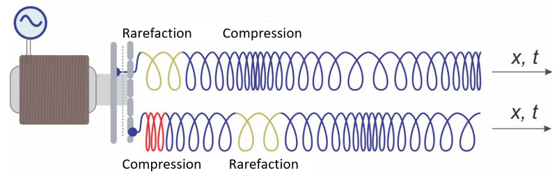
Figure 3: Formation of a longitudinal wave
The buzzer's anchor is a pendulum that oscillates harmonically from the extreme left to the extreme right position, as shown in the graph in Figure 4 below. During oscillation, it decompresses and compresses the spring. The density of the rings changes and rarefactions and compressions are formed on the spring, depending on the direction in which the buzzer anchor is moving. The rarefactions and compressions then travel along the spring.
Let's take a closer look at Figure 3:
Moving the buzzer anchor to the left means that the spring rings will move apart. Next to the anchor, there will be an area with a low density of rings on the spring. We also call it the rarefaction area - the yellow area in figure 3 above.
As the anchor moves to the right, it causes the coils of the spring to compress, resulting in a high density of rings on the spring. It is called the compression area - the red area in Figure 3 above. Meanwhile, the previous rarefaction will have already moved along the spring to the right.
The oscillation of the anchor according to Figure 3 is harmonic and is described by the equation:
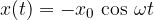
Let's explain why we chose such an equation. Since the pendulum (anchor) is in the extreme position at the beginning of the observation, we chose the "cosine" function. The anchor is initially at the extreme left and has a negative displacement amplitude, so the cosine is multiplied by a negative amplitude  . In the graph in Figure 4, we can see that the oscillation angle of the anchor and the ring density have the same initial shape. We say that they are in phase.
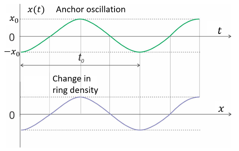
Figure 4: Anchor oscillation and ring density
Let's imagine that we are photographing the waves on the spring at a certain moment when the anchor is in the extreme left position - see Figure 5 below. Let's see how the density of the rings changes as we move along the spring to the right in the figure.
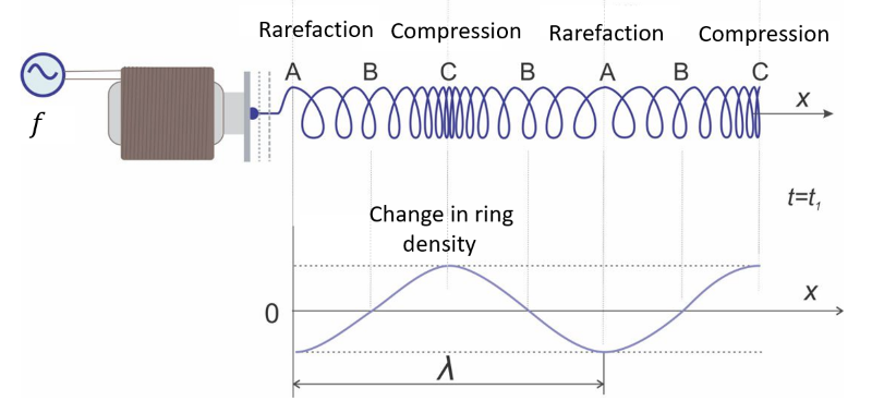
Figure 5: Graph of the change in the density of the rings in the spring depending on the position x along the spring
We labelled some areas on the spring in Figure 5:
Rarefaction A: Rarefaction occurs next to the buzzer when the anchor is in the extreme left position and tensioning the spring. It repeats along the spring at each wavelength  . The density of the spring rings is the lowest there.
Compressions C: The compression in our example is half a wavelength from the origin and repeats every wavelength. The density of the spring rings is highest there.
Neutral position B: Between the extreme positions A and C of the anchor is the neutral or equilibrium position B. There the density of the rings is as it would be in a spring on which there is no wave.
Compressions and rarefactions are transmitted forward from the source by means of the oscillation of the spring particles. The energy carried by the wave also depends on the amplitude of this oscillation.
Let's first draw the spring in its equilibrium position, when its shape is still unchanged - Figure 6 A. Then we draw the vibrating spring - Figure 6 B. The observed moment is when the anchor moves to the extreme left position and creates a rarefaction at the beginning of the spring.
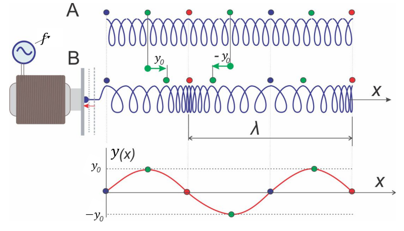
Figure 6: Displacement from equilibrium position along the spring in the observed time
Let's see what the position of the individual areas is with respect to the equilibrium position on the spring. For easier observation, we mark the areas with dots in the figure:
rarefaction - marked with a blue dot
neutral position - marked with a green dot
compression - marked with a red dot
neutral position - marked with a green dot
etc.
We can see that the part of the spring marked with a green dot has the largest displacement from the equilibrium position. There, the density of the rings is the same as for an undeformed spring (neutral position). So the displacement amplitude  is at this point. The displacement is zero when there is a rarefaction or compression on the spring.
Now let's combine the graphs of the density of rings and the displacement from the equilibrium position from figures 5 and 6. The graphs are in figure 7. The chosen moment of observation is when the anchor is on the far left side.
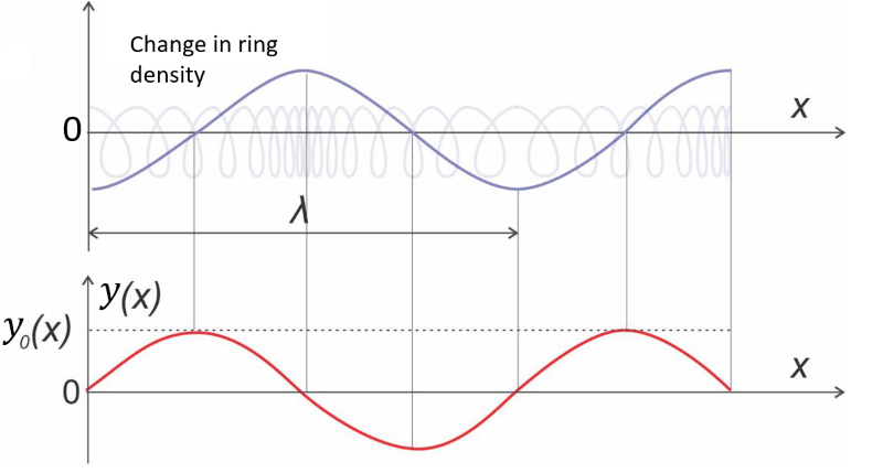
Figure 7: Graph of spring density and displacement from equilibrium
From the figure, we see that the displacement from the equilibrium position is the amplitude  when the coil is at the neutral position and that the displacement is zero in the case of compression and rarefaction.
Where the ring density graph passes through zero (the density node) is the peak of the displacement from the equilibrium position (neutral position). Or vice versa, where the ring density graph is displaced by , the displacement from the equilibrium position is zero (compression and rarefaction).
Compressions and rarefactions propagate from the source along the spring at a velocity . At the time of  , they travel a distance
  . In one oscillation period
  , they travel a distance equal to the wavelength of the wave:

We note that the period is the reciprocal of the frequency  :
:

Therefore:
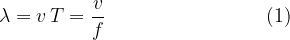
At a given frequency , the wavelength will depend only on the speed of the wave. From equation 1, we therefore have:

The deviation of the particles from the equilibrium position depends on the time  of the observation and the position
  on the string. We denote it by the function notation
  .
.
Let us first describe the displacement of the particles depending on the position on the spring, i.e.  . The wave is observed at the time
  when the anchor is at the extreme right.
The function that describes the displacement at time depending on the position is given as:
The function that describes the displacement at time depending on the position is given as:
At time  , the wave moves along the spring by
  , as shown in Figure 8 below.
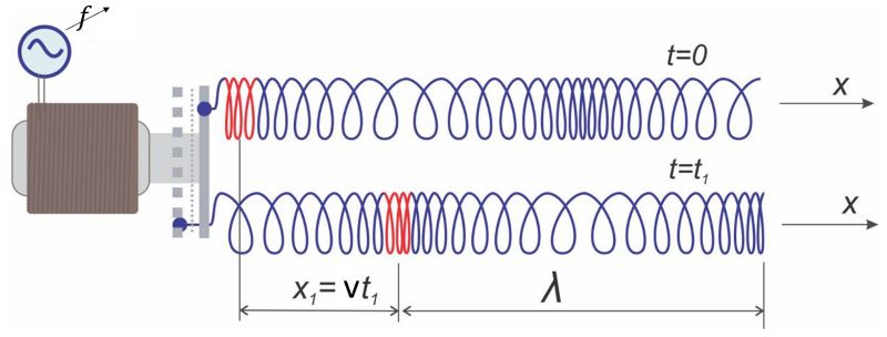
Figure 8: Formation of a travelling longitudinal wave
In the equation derived above, let us consider this shift or time lag.
The function that describes the displacement as a function of the position  and time
  is given as:
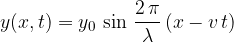
We have obtained an equation that represents the relationship between the displacement  of a particle (e.g. a spring) from its equilibrium position as a function of time and distance . Let's draw a graph - Figure 9:
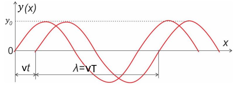
Figure 9: Graph of function 
A progressive longitudinal wave can be expresses by the equation: