Personal collections

In the chapter, Sound waves, we learned about the formation of a sound wave: when moving a membrane, the sound element compresses or expands air molecules or some other substance that transmits sound. The compressions and rarefactions are then propagated towards the receiver. The particles of the substance are thus forced to oscillate with a frequency determined by the source of the sound.
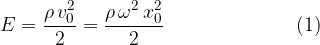
Sound energy is the energy of the oscillating particles. Molecules of matter behave similarly to a flexible spring. When they are compressed (increased pressure), all the sound energy is in elastic energy. As the molecules expand, the elastic energy decreases, and the kinetic energy increases. In the equilibrium position (that is, at mean air pressure) all the energy is in the kinetic energy of the molecules.
As with the spring pendulum, also for the oscillation of molecules in matter, the total energy  of oscillation is equal to the sum of the kinetic energy
  and elastic energy
  . The total energy is constant and equal to the maximum elastic energy
  or maximum kinetic energy
  :
:

Let's observe the longitudinal oscillation of a molecule with mass  . Its kinetic energy
  is:
is:

From the kinetic energy, we can derive the kinetic energy density as follows:
The maximum velocity  of oscillation is given as:

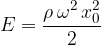
When the maximum velocity is inserted into the sound energy density , we get the total (maximum) energy density . This is also the sound energy density:
We can see that the higher the density of a substance, the higher the sound energy density. Sound therefore has much greater energy in metal than air at the same distance from the equilibrium position and the same frequency.
The sound power  is its energy
  in the observed time
  :
:
If we divide the power by the cross-sectional area  , we get the sound power density or sound intensity
  :
:

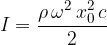
The sound intensity is derived from the formula above as follows:
The sound intensity (sound power density) is therefore the sound energy density multiplied by the speed of sound propagation  .
.
We note from equation 1 above that:
Therefore, the sound intensity is:
The sound that we can hear is located in the sound intensity range between  and
and  watt per square metre:

The lowest sound intensity that we can still hear is called the hearing threshold. The hearing threshold depends on the frequency of the sound. The human body is most sensitive to a frequency of about  .
.
At other frequencies that humans can hear ( to about
  ), a higher sound instensity is required. Also, the audibility of higher frequencies in particular decreases with age.
The maximum sound intensity is limited by the pain threshold.
The feeling of sound - that is, the auditory intensity of the sound - is not proportional to the density of the sound power, but to its logarithmic ratio:
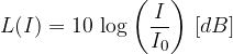
The unit for sound intensity is the decibel [dB].  is the lower hearing threshold and
  is the pain threshold.
From the above notation, we see that sound intensity level is a logarithmic function. But if we want a straight line as a graph, we have to apply logarithmic values to the abscissa. The sound intensity level graph is therefore a linear function of the decimal logarithm, which has in its argument the ratio of the observed sound intensity and the audibility threshold (Standard reference sound intensity) at 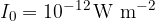 .
.
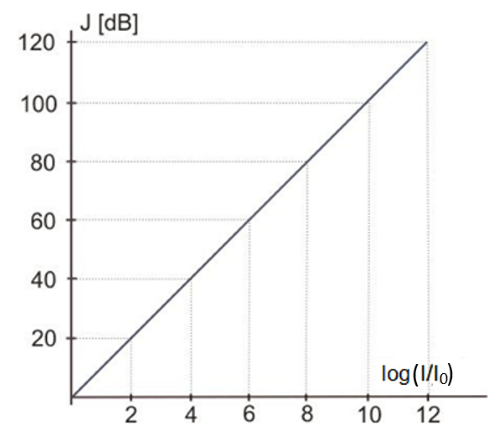
Sound intensity level graph in logarithmic scale
A speaker emits a sound that contains several frequencies at the same time. Sound is transmitted to our ears via longitudinal air waves. We can hear it, but we can also see sound waves, e.g. by recording it with a microphone and looking at it on an oscilloscope. In this case, the air waves are converted into an electrical signal with the same form as the sound signal. On the oscilloscope, we see the shape of the wave, that is, how the wave changes with time. So we see the time function  of the deviation from the equilibrium position of the longitudinal air wave, converted into an electrical signal.
If we look at a sound recording, we see that the wave is still periodic, but it does not have a sinusoidal shape. We already know that a non-sinusoidal waveform contains higher harmonic components, but we don't see from the picture what their magnitude is - see the examples below. But, if we look at a recording of noise, we see a completely random function of time, but we do not see which frequencies are contained in this noise and how they are emphasized.
In order to determine which frequencies a sound or noise is made of, we need to do a frequency or spectral analysis. It can be made directly from the given time waveform . For this purpose, a slightly more complex mathematical tool called Fourier analysis is used. We have not yet mastered this mathematical tool, but we can still use it. It is an integral part of many computer programs designed for sound analysis.
The results of the analysis are usually presented in the form of a graph. The graph has:
the angular speed or frequency on the abscissa, and
on the ordinate axis we can write:
the calculated or measured proportion of the power that a sound has in a narrow frequency range around a selected frequency:
It is called the spectral power density.
sound intensity in the narrow observed frequency band:
It is called the spectral density of the sound power.
Most often, the scale on the ordinate (y-axis) of the spectrum graph is written in decibels - dB. But what are decibels?
In the previous chapter, we learned what sound intensity level is, expressed in decibels. A similar equation as for sound intensity level also applies more generally. In our case, we get a scale in decibels if we compare the spectral power density with some reference value  (e.g. the spectral power density of the fundamental tone), logarithmize and multiply by 10:
Sound waves can have:
discrete spectrum
A discrete spectrum has portions of energy only at certain frequencies. The discrete spectrum has e.g. sound. In the sound spectrum, there are vertical spectral lines only at the frequencies that make up the sound.
continuous spectrum
The continuous spectrum has a non-periodic wave. This is, for example, noise or bang. Both contain an infinite number of frequencies. In this case, the spectrum is a continuous function - a curve or line that shows the dependence of  .
.
The sound spectrum can also be measured. That is why we use specialized electronic instruments - spectrum analyzers or one of the many computer programs designed for sound synthesis (sound generator) and its analysis.