Personal collections

Motion is the change in the position of a body over time. A body can move around:
lines (1-dimensional space);
plane (2-dimensional space);
space (3-dimensional space).
Depending on the speed, we divide motion into:
uniform motion (speed is constant);
non-uniform motion (speed is not constant but changes over time).
Depending on the path of the motion, we divide the motion into:
linear (straight) motion;
non-linear (curved) motion.
A moving body makes a journey. We must distinguish between the concept of a path (denoted by e.g.  ) and the position of the body (denoted e.g. by
  ). During motion, the distance we cover increases with time. This does not apply to our location. The position is usually defined as the distance to the point where starting point of our journey is.
For uniform motion, the distance traveled by the body is equal to the product of its speed  and time
  :
:

In equation (1), when we write , we really have in mind the distance travelled, which means that we are interested in the difference between the final and starting point on the motion path:

where  is the point where we stop measuring the distance and
  is the point where we start measuring the distance (see Figure 3). In order to emphasize that it is the difference between the end point and the starting point, in equation (1) we write
  instead of , or:
The same goes for time:

where  is the point where we stop measuring time and
  is the point where we start measuring time (see Figure 3). Therefore, in equation (1) we also replace time with
  :
:
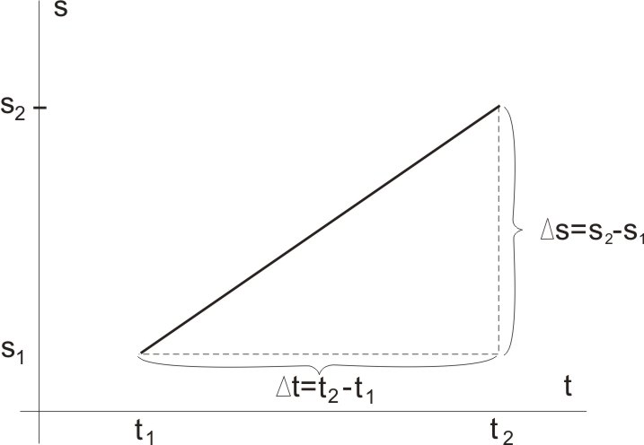
Figure 3: Distance-time graph of a linear motion
Equation (1) is written in general form as the change in position in the observed time :

Let's also make the speed the subject of the formula:

In most cases, we have to use the base units of measurement in the tasks, i.e. the unit of distance is metre ( ), the unit of time is second (
 ) and the unit of speed is therefore metres per second (
 ). If the quantities are in some other unit, we first convert them to the base units when solving the exercises.
Let's observe the linear motion in an x, y coordinate system. The initial distance from the coordinate origin is denoted by  , and the time when the body starts to move is denoted by
  . Let's observe how the distance of the object from the coordinate origin changes with time . Since this is a linear motion, the distance from the origin varies linearly with time.
Let's write equation 2 again:
The dependence of the distance of an object from the coordinate origin on the observed time is written with the general equation:
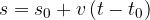
where:
 is the distance of the object from the coordinate origin at the beginning of the motion.
 the time when the body begins to move.
Let's first place the object in the coordinate origin and see how its distance changes with time. We use equation (2) and consider that the initial distance is zero and the time when the object starts moving is also zero. We write equation (3):

The graph of the described motion is in Figure 4. The speed of the motion determines the slope of the line. If the speed is higher, the steepness of the line will be higher, which means that the body will move further away from the starting point in the same time.
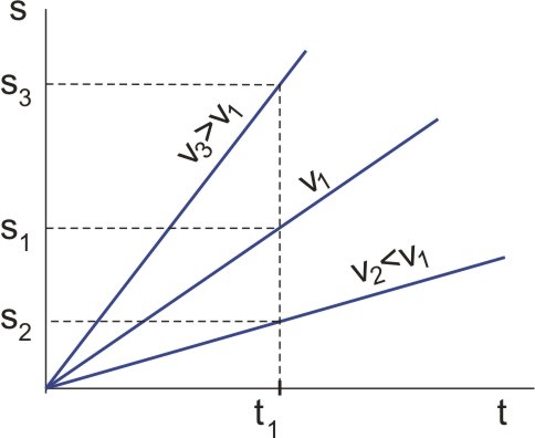
Figure 4: A body moving uniformly away from the starting point
The object is located at a distance from the coordinate origin, and we begin to observe the approach of the object to the coordinate origin at time .
Equation (3) in this case becomes:

Since the object is approaching, the sign of the velocity is negative (and vice versa: the velocity is positive if the object is moving away), the graph of  is a decreasing function and is as shown in Figure 5 below.
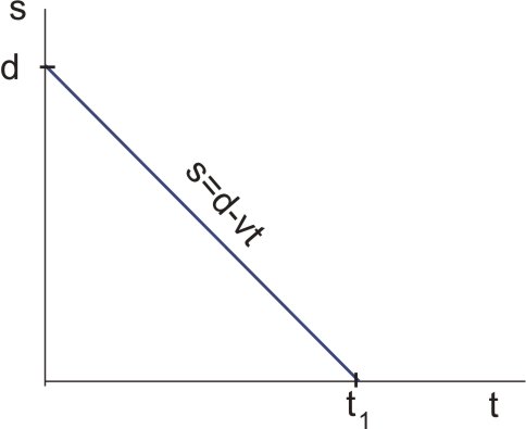
Figure 5: Object approaching the coordinate origin
When does the object arrive at the coordinate origin?
Let's use the equation:
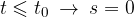
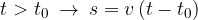
What if the object is located at the starting point and starts moving in time  ?
?
We will now divide the distance formula into two intervals:
Did we write the second equation correctly? Let's check:
If we insert  into the equation, the distance must still be zero, because that's when the object started to move:
Only when  is
is  ; the body begins to move away from the starting point.
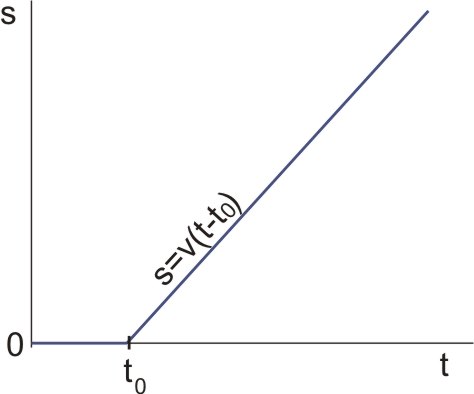
Figure 7: start of movement with time delay
A body moves for a certain time with speed  , then with another speed
  , etc. This is a sectional uniform motion. It moves uniformly in each section, but the speed of motion varies from section to section.
To make it easier to imagine such a motion, let's draw the graph of speed against time.
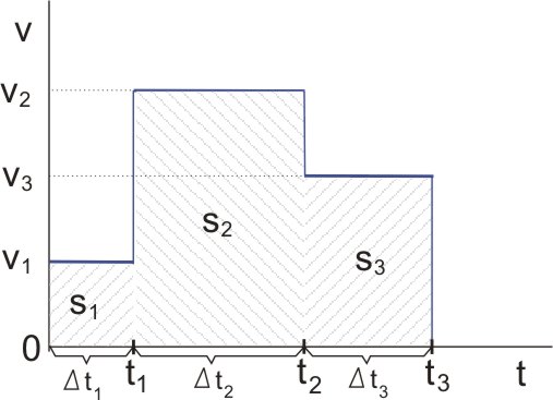
Figure 9: Speed-time graph of a sectional uniform motion
Sections of uniform motion are represented in Figure 9 by straight lines parallel to the time axis. The speed is constant in each section.
Let's look at the first section in Figure 9. The body moves with a speed from 0 seconds to  seconds. Let's calculate the distance using the well-known equation:

Graphically, we imagine the distance as a rectangle shaded with diagonal lines in Figure 9. Similarly, we could calculate the distance for all three sections according to Figure 9:


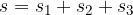
The total distance travelled is therefore:
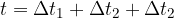
The distance was completed in seconds:
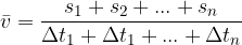
The average speed  of the body, however, is the total distance divided by the total time:

The average velocity of a body is the velocity that the body would have to have if it were moving uniformly all the time in order to cover the same distance in the same time as in sectional uniform motion.
We calculate it by summing all the distances and dividing by the total time:
A body moves straight and uniformly in a direction and with the speed of the resultant of two or more Motion velocity vectors. Depending on the type of task and our knowledge of mathematics, vectors can be added graphically, geometrically, or with the help of angular functions. With advanced knowledge of mathematics, we can also use vector calculus (see Operations with vectors).
Let's take a look at an example of how we solve tasks where speed consists of several components.