Personal collections

In the chapter, Uniform motion, we studied a body moving at a constant speed along a straight line. We called this motion linear uniform motion.
But in general, the speed of motion is not constant but changes with time. In this case, the motion is non-uniform.
Figure 1 shows the speed-time graph of a body for some non-uniform motion, where the body's speed changes in sections. If its speed increases, we speak of acceleration, but if it decreases, the acceleration is negative and we call it deceleration.
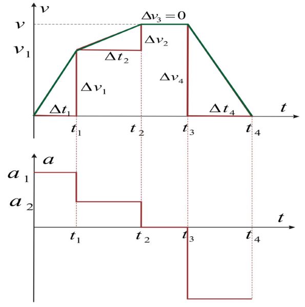
Figure 1: Non-uniform motion in sections
The magnitude of the acceleration (or deceleration) depends on the change in speed during the observed time:
The unit of acceleration is:

Let's go back to Figure 1. We know from mathematics that the slope of a line is calculated using the formula:

If we look at the graph above in Figure 1, we have labelled the x-axis with  (the x-axis represents time) and the y-axis with
  (the y-axis represents the speed). Let's write down the equation for the slope again, with the symbols from Figure 1:

We got nothing but equation (1), which means that the acceleration on the graph at the top in Figure 1 is exactly the slope of the individual lines. This can be clearly seen in comparison with the graph below in Figure 1: the lower the slope of the line (in the graph at the top), the lower the acceleration (in the graph below in Figure 1).
In the graph below in Figure 1, we can also see that:
during the time interval  the speed does not change, so the acceleration is zero.
during the time interval  the velocity decreases, so the acceleration is negative. We call it deceleration.
The acceleration of motion is the change in the speed of motion in the observed time:
The acceleration of a body is obtained by observing the slope (slope) of the graph of the function  .
.
The unit of acceleration is:
The calculations in this chapter are intended for students with advanced knowledge. The reader can skip this chapter without any effect on the understanding of the rest of the material.
In most real situations, however, the speed changes continuously (more smoothly and not in sections as in Figure 1). A somewhat more realistic graph of speed and acceleration is shown in Figure 2 below:
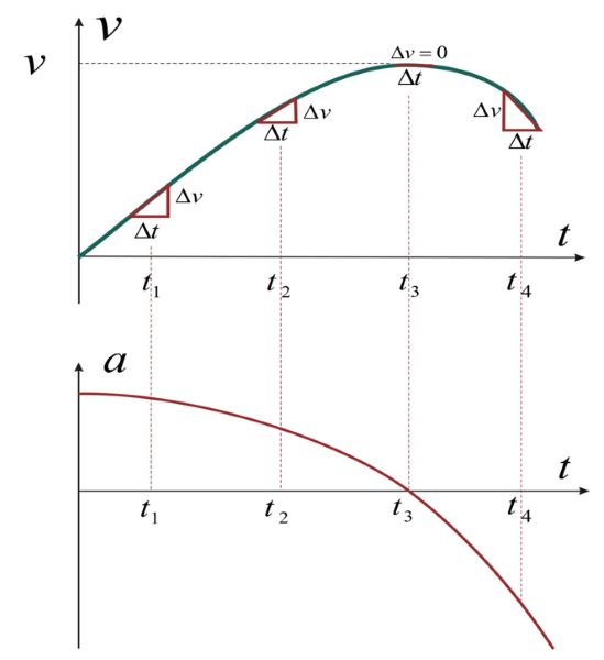
Figure 2: General non-uniform motion
First, let's describe what is happening in Figure 2: the acceleration is initially positive and decreases. Therefore, the slope  decreases from
  to
to  . At time
  , the acceleration is zero because the slope is zero. In time
  , the slope is negative - the graph of decreases with time.
We calculate the acceleration of such a general curve as follows: when observing the slope of the curve, we take sufficiently small sections of the observation  , so that we can consider that the speed within changes linearly. But this happens only when the observed interval decreases towards an infinitely small value (but never reaches the value 0). This is actually just the derivative of the function after time :

The equation is very similar to equation (1), but to emphasize that we are talking about infinitesimally small differences, we use the notation  (d difference ) instead of
  in the equation.
Uniformly accelerated motion is a special case of non-uniform motion, where the acceleration  is the same (constant) all the time. In uniformly accelerated motion, velocity varies linearly with time.
We start from equation (1):
The general equation for uniformly accelerated motion (that is when the acceleration is constant) is:

Let's look at some special examples of uniformly accelerated motion.
Let us consider the special case of the equation:
when the initial velocity  , and the time
  when we start measuring the motion is set to 0. The equation therefore becomes:

We can notice that we have obtained an example of a linear function, where the constant  is equal to 0; we start drawing the line from the origin, and the slope gives the acceleration :
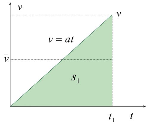
Figure 3: Graph of a body accelerating at an initial speed of zero
From the graph, we can read the time  at which the body reaches its final speed , so we can write the acceleration as:

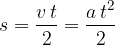
Let's calculate the distance travelled. During the time interval  to , the speed varied from to . During this time, the body travels a distance
  equal to the product of the average speed
  and time :
We generalize the resulting equation by expressing the distance as  and time as :
Equation (4) represents a quadratic function. In uniformly accelerated motion, the distance travelled varies with the square of time. Let's see:
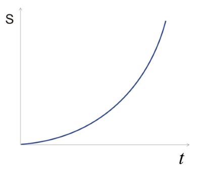
Figure 4: The distance-time graph is a parabola
From equation (3) we can obtain a formula for the time when the body completes the distance  :
:
The final speed is given as:
Let's generalize the expression. The time taken by the body to travel a distance is given as:

The final speed in terms of the distance of the body is given as:

In a uniformly accelerated motion with an initial velocity of zero, it is considered that:
the speed in terms of the time is given as:
the distance covered by the body is given as:
the time taken to cover distance  is given as:
the speed in terms of the distance  is given as:

When calculating the distance travelled by a uniformly accelerated body in time , we need the average speed of the body in the measured time. Without going into a more detailed calculation at this point, let's just write down the average speed of the body that has the initial speed  at the start of the measurement and reaches the final speed :

If the initial speed , then:
 )
)The distance travelled by a uniformly accelerated body can also be calculated using a graph; let's look at Figure 3. The area under the graph (the region is coloured green) is exactly the same as the distance travelled. This conclusion also applies in general:
The distance in any (uniform or non-uniform) motion is obtained by calculating the area under the velocity-time graph.
Let's calculate the area. We can see that the green area in Figure 3 is a triangle. The area of a triangle is half base times the height. If we map this to our example, we again get:

Let us consider a special case of the equation:
where the body has an initial speed at the beginning of the measurement, and the times when we start measuring the motion is set to 0. The equation therefore becomes:

We can see that we have obtained an example of a linear function, where the constant is equal to . As we know, the constant tells us where the graph intersects the y-axis. Therefore, we start drawing the graph at point , and the slope gives the acceleration :

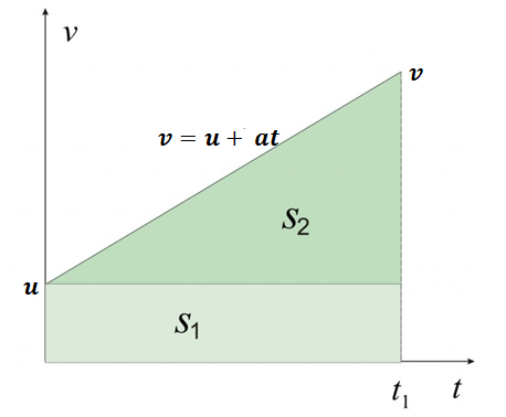
Figure 5: Graph of an accelerating motion with initial speed
The distance travelled by the body in time is equal to the area under the velocity-time graph (see Figure 5). It consists of the distance that the body would travel if it were moving at a constant speed and the component of uniformly accelerated motion.
The equation can be written more generally by expressing the distance as a function of any observed time:

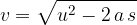
Let's also calculate the velocity as a function of the distance with the known acceleration and the initial velocity :
In uniformly accelerated motion with an initial velocity , it is noted that:
the velocity acquired by a body at time can be calculated using the following two equations:

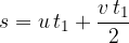
the distance travelled by the body in time  is given as:
When calculating the distance that a uniformly accelerated body completes in time , we will need the average speed of the body in the measured time. Without going into a more detailed calculation at this point, let's just write down the average speed of a body that has an initial speed at the start of the measurement and reaches the final speed :

This is actually the arithmetic mean of the initial and final velocities.
As before, when we calculated the distance travelled by a uniformly accelerated body, we can now calculate the distance using a graph; let's look at Figure 5. The area under the velocity-time graph (the area is coloured green) is exactly the same as the distance travelled. The area under the graph consists of a rectangle and a triangle:

The area of both sections is easily identifiable; the area of the rectangle is:

and the area of the triangle is:

We insert both areas and get the already known formula again:
At the start of the measurement, the body has an initial velocity . As the body moves with constant deceleration, the body's speed decreases. We also say that the body decelerates. Let's see how the graph of velocity-time graph () looks like:
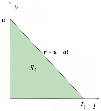
Figure 6: Graph of the motion of a body with a decreasing initial velocity
The acceleration of such motion is negative (see Figure 6). We also call it a deceleration. Let's obtain the formula for deceleration:
Acceleration is negative. We call it deceleration.
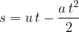
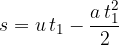
The formulas for velocity and distance are the same as in the previous chapter. We only consider that the acceleration is negative.
The speed in terms of time is given as:

The distance in terms of time is given as:
The speed in terms of the distance at a given acceleration is given as:
Let's obtain the time when the speed drops to zero:
Therefore, the time required to stop the body is:

The maximum distance it travels before stopping is equal to the area under the velocity-time graph - Figure 5.
The formulas for uniformly decelerating motion with an initial velocity are the same as the formulas for uniformly accelerated motion, only the acceleration has an accompanying sign and appears in the formulas with a minus sign ( ):
):
the velocity of the body is calculated using the following two formulas:
the distance that the body travels in time is given as:
the time at which the body stops is given as:
the stopping (or braking) distance is given as: